Two_Node_Process
Scott Koermer
2022-06-17
Source:vignettes/Two_Node_Process.Rmd
Two_Node_Process.RmdThe function BMB is used with a two node process and
simulated data.

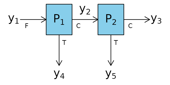
The constraints around these process nodes are:
\[\begin{align} y_1 &= y_2 +y_4\\ y_2 &= y_3 +y_5 \end{align}\]
Therefore the matrix of constraints, C is:
C <- matrix(c(1,-1,0,-1,0,0,1,-1,0,-1), nrow = 2, ncol = 5, byrow = TRUE)
C
#>      [,1] [,2] [,3] [,4] [,5]
#> [1,]    1   -1    0   -1    0
#> [2,]    0    1   -1    0   -1
The constrainProcess function in the
BayesMassBal package is used to generate an X
matrix based on C that will later be used with the
BMB function.
X <- constrainProcess(C = C)
X
#>      [,1] [,2] [,3]
#> [1,]    1    1    1
#> [2,]    1    0    1
#> [3,]    1    0    0
#> [4,]    0    1    0
#> [5,]    0    0    1
Constraints can also be imported from a .csv file. The
path to a file, included in the BayesMassBal package, for
this process can be found and constraints can be imported by specifying
the location for the file argument for
constrainProcess as shown below:
constraint_file_location <- system.file("extdata", "twonode_constraints.csv",package = "BayesMassBal")
X <- constrainProcess(file = constraint_file_location)
The previously simulated data is loaded from a .csv file
using the importObservations() function. The local location
of the the file imported below can be found by typing
system.file("extdata", "twonode_example.csv",package = "BayesMassBal").
View the document in Excel to see how your data should be formatted for
import. Note: it is not required that the
entries into the *.csv file are separated by
";".
y <- importObservations(file = system.file("extdata", "twonode_example.csv",
                                  package = "BayesMassBal"),
                  header = TRUE, csv.params = list(sep = ";"))
Then, the BMB function is used to generate the
distribution of constrained masses from the data with
cov.structure = "indep".
indep.samples <- BMB(X = X, y = y, cov.structure = "indep", BTE = c(100,3000,1), lml = TRUE, verb = 0)The output of BMB is a BayesMassBal object.
Special instructions are designated when feeding a
BayesMassBal object to the plot() function.
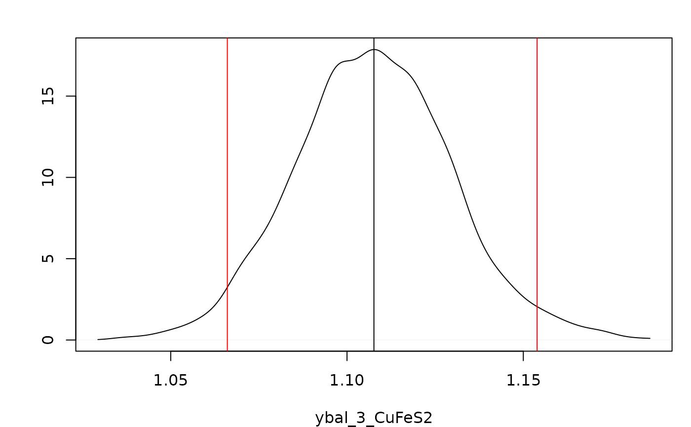
Adding the argument layout = "dens" and indicating the mass
balanced flow rate for CuFeS2 at \(y_3\) should be plotted using a list
supplied to sample.params, the desired distribution can be
plotted with its 95% Highest Posterior
Density Interval.
plot(indep.samples,sample.params = list(ybal = list(CuFeS2 = 3)),
    layout = "dens",hdi.params = c(1,0.95))
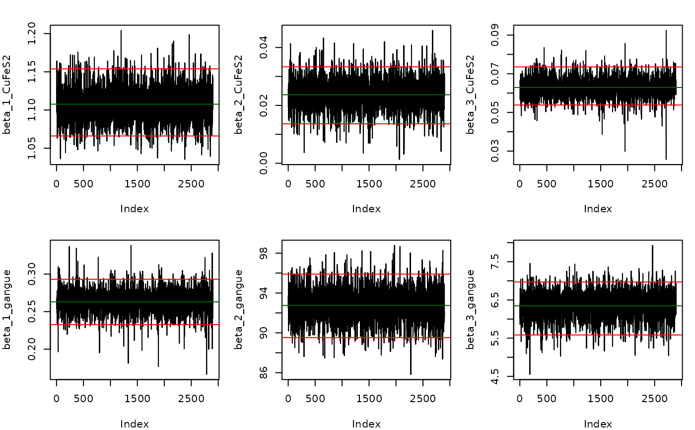
It is also possible to generate trace plots to inspect convergence of the Gibbs sampler. Here are trace plots for \(\beta\)
plot(indep.samples,sample.params = list(beta = list(CuFeS2 = 1:3, gangue = 1:3)),layout = "trace",hdi.params = c(1,0.95))
A quantitative diagnostics for convergence and autocorrelation are
available as part of the output from BMB:
indep.samples$diagnostics
#> $beta
#> $beta$CuFeS2
#>   index         cd      ess
#> 1     1 -0.3611161 2523.569
#> 2     2  0.7828321 2900.000
#> 3     3 -0.7725090 2701.475
#>
#> $beta$gangue
#>   index         cd      ess
#> 1     1  2.7234190 2664.632
#> 2     2  0.9959390 2900.000
#> 3     3 -0.2814149 1884.572
#>
#>
#> $Sig
#> $Sig[[1]]
#>   index          cd      ess
#> 1     1  0.07827022 2629.087
#> 2     2  0.28976726 2900.000
#> 3     3 -0.92940701 2470.207
#> 4     4 -1.20257978 2184.124
#> 5     5 -0.04802145 1791.077
#>
#> $Sig[[2]]
#>   index         cd      ess
#> 1     1 -0.3968014 2900.000
#> 2     2  0.4150925 2666.449
#> 3     3 -1.6538871 1495.024
#> 4     4  0.5935790 2235.558
#> 5     5  0.5005302 2259.714
The model with independent variances may not be the best fitting model. Models specifying covariance between sample locations for a single component, and covariance between components at a single location are fit.
component.samples <- BMB(X = X, y = y, cov.structure = "component", BTE = c(100,3000,1), lml = TRUE, verb = 0)
location.samples <- BMB(X = X, y = y, cov.structure = "location", BTE = c(100,3000,1), lml = TRUE, verb = 0)Computing \(\log(\mathrm{Bayes Factor})\) for \(BF = p(y|\texttt{indep})/p(y|\texttt{component})\):
indep.samples$lml - component.samples$lml
#> [1] -126.8253
Then comparing \(p(y|\texttt{component})\) to \(p(y|\texttt{location})\)
component.samples$lml - location.samples$lml
#> [1] 0.8157781
Shows there is little difference between the models where
cov.structure = "location" and
cov.structure = "component", but both of these models
better explain the data than cov.structure = "indep".
We can view a summary of the favored model by passing a
BayesMassBal object to the summary function.
While not done in this case, the summary table can be saved by passing
the desired name of a *.csv file to the export
argument.
summary(component.samples, export = NA)
#> Mass Flow Rates:
#>
#> CuFeS2:
#> --------------------
#>  Sampling Location Expected Value     95% LB     95% UB
#>                  1     1.19726816 1.14701389 1.24590566
#>                  2     1.17185264 1.12298323 1.21825816
#>                  3     1.10912627 1.05847094 1.15974298
#>                  4     0.02541552 0.01738181 0.03464440
#>                  5     0.06272637 0.05340892 0.07369845
#>
#> gangue:
#> --------------------
#>  Sampling Location Expected Value     95% LB      95% UB
#>                  1    100.1924885 95.4304044 104.9670533
#>                  2      6.6586282  5.7752361   7.3926409
#>                  3      0.2600511  0.2251857   0.2914376
#>                  4     93.5338603 89.0256219  98.0016813
#>                  5      6.3985771  5.5321841   7.1303883
#>
#> Total:
#> --------------------
#>  Sampling Location Expected Value    95% LB     95% UB
#>                  1     101.389757 96.520067 106.040748
#>                  2       7.830481  7.071272   8.696424
#>                  3       1.369177  1.308046   1.429046
#>                  4      93.559276 89.047376  98.021858
#>                  5       6.461303  5.589737   7.185424
#>
#>
#> log-marginal likelihood:
#> -66.0586924576421
The main effect of a variable independent of the process can be
calculated by supplying a function, fn that takes the
arguments of mass balanced flow rates ybal, and the random
independent and uniformly distributed variables x.
Information can be gained on the main effect of a particular element of
x, xj, on fn using the
mainEff function. Output from mainEff includes
information on the distribution of \(E_x\lbrack f(x,y_{\mathrm{bal}})|x_j
\rbrack\).
fn_example <- function(X,ybal){
      cu.frac <- 63.546/183.5
      feed.mass <- ybal$CuFeS2[1] + ybal$gangue[1]
      # Concentrate mass per ton feed
      con.mass <- (ybal$CuFeS2[3] + ybal$gangue[3])/feed.mass
      # Copper mass per ton feed
      cu.mass <- (ybal$CuFeS2[3]*cu.frac)/feed.mass
      gam <- c(-1,-1/feed.mass,cu.mass,-con.mass,-cu.mass,-con.mass)
      f <- X %*% gam
      return(f)
      }

rangex <- matrix(c(4.00 ,6.25,1125,1875,3880,9080,20,60,96,208,20.0,62.5),
                   ncol = 6, nrow = 2)
mE_example <- mainEff(indep.samples, fn = "fn_example",rangex =  rangex,xj = 3, N = 25, res = 25)
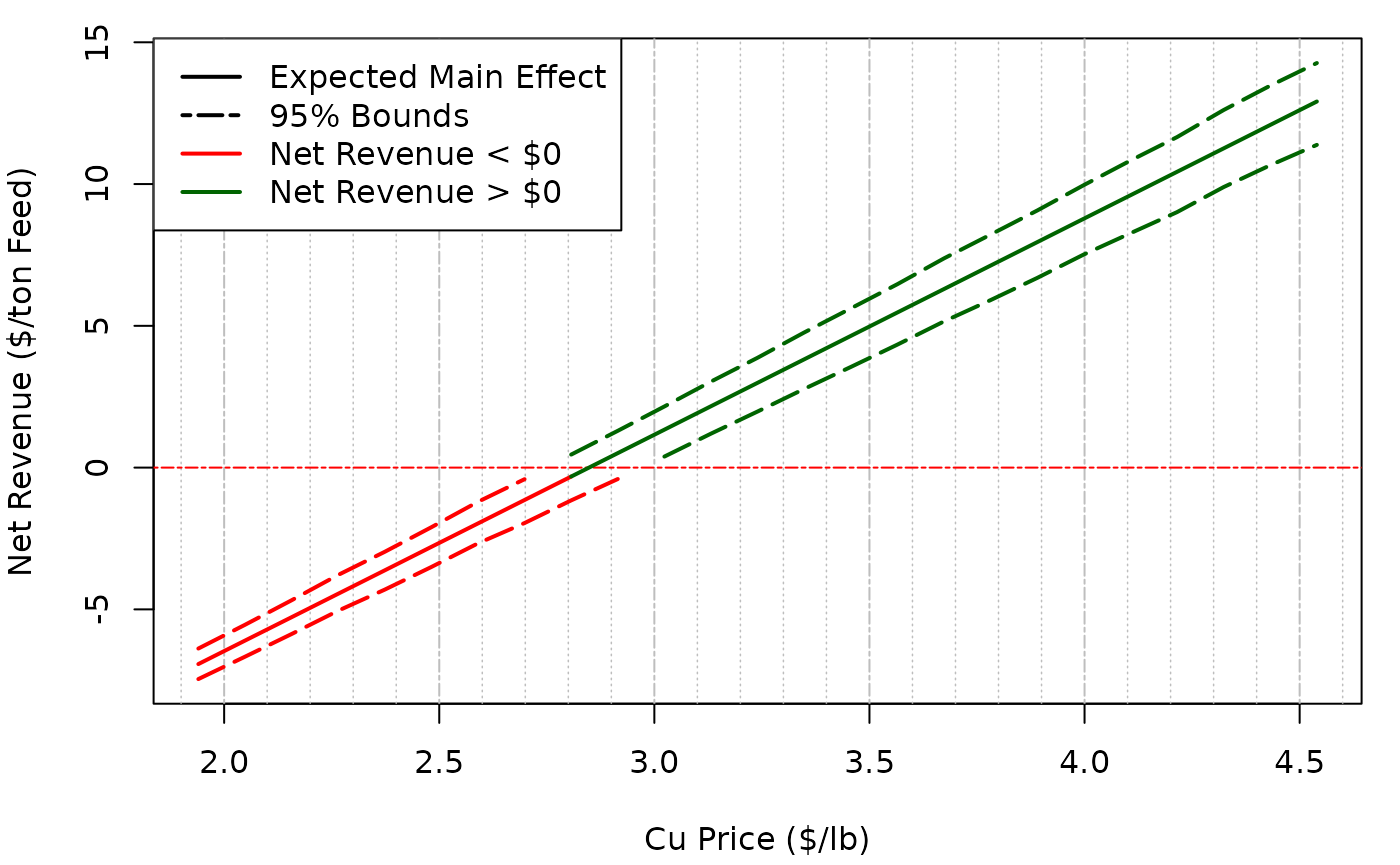
A plot of the output can be made. To get lines that are better
connected, change increase N in the mainEff
function.
m.sens<- mE_example$fn.out[2,]
hpd.sens <- mE_example$fn.out[c(1,3),]
row.names(hpd.sens) <- c("upper", "lower")
g.plot <- mE_example$g/2000

y.lim <- range(hpd.sens)

lzero.bound <- apply(hpd.sens,1,function(X){which(X <= 0)})
lzero.mean <- which(m.sens <= 0)

main.grid <- pretty(g.plot)
minor.grid <- pretty(g.plot,25)
minor.grid <- minor.grid[-which(minor.grid %in% main.grid)]

y.main <- pretty(hpd.sens)

opar <- par(no.readonly =TRUE)
par(mar = c(4.2,4,1,1))
plot(g.plot,m.sens, type = "n", xlim = range(g.plot), ylim = y.lim, ylab = "Net Revenue ($/ton Feed)", xlab=  "Cu Price ($/lb)")

abline(v = main.grid, lty = 6, col = "grey", lwd = 1)
abline(v = minor.grid, lty =3, col = "grey", lwd = 0.75)

abline(h = 0, col = "red", lwd = 1, lty = 6)

lines(g.plot[lzero.mean],m.sens[lzero.mean],col = "red", lwd =2)
lines(g.plot[-lzero.mean[-length(lzero.mean)]],m.sens[-lzero.mean[-length(lzero.mean)]],col = "darkgreen", lwd =2)

lines(g.plot[lzero.bound$lower],hpd.sens[2,][lzero.bound$lower], lty = 5, lwd = 2, col = "red")
lines(g.plot[-lzero.bound$lower],hpd.sens[2,][-lzero.bound$lower], lty = 5, lwd = 2, col = "darkgreen")

lines(g.plot[lzero.bound$upper],hpd.sens[1,][lzero.bound$upper], lty = 5, lwd = 2, col = "red")
lines(g.plot[-lzero.bound$upper],hpd.sens[1,][-lzero.bound$upper], lty = 5, lwd = 2, col= "darkgreen")

legend("topleft", legend = c("Expected Main Effect", "95% Bounds", "Net Revenue < $0", "Net Revenue > $0"), col = c("black","black","red", "darkgreen"), lty = c(1,6,1,1), lwd = c(2,2,2,2), bg = "white")
par(opar)